このシリーズでは物体検出でお馴染みのYOLOシリーズの最新版「YOLOX」について、環境構築から学習の方法までまとめます。
YOLOXは2021年8月に公開された最新バージョンであり、速度と精度の面で限界を押し広げています。
第6回目である今回は、YOLOXの後処理の活用例としてモザイク処理の自動化を実装する方法を紹介します。
Google colabを使用して簡単に物体検出のモデルを実装することができますので、ぜひ最後までご覧ください。
今回の目標
・YOLOXの後処理
・モザイク処理
・YOLOXによるモザイク処理の自動化
物体検出の活用
物体検出では物体の座標を出力することができます。
この座標情報と画像処理を組み合わせることで物体検出の活用の幅が広がります。
今回はモザイク処理を例にして実装方法を紹介します。

YOLOXの導入
早速実装していきましょう。
以下、Google colab環境で進めていきます。
まずはGPUを使用できるように設定をします。
「ランタイムのタイプを変更」→「ハードウェアアクセラレータ」をGPUに変更
今回紹介するコードは以下のボタンからコピーして使用していただくことも可能です。
![]()
YOLOXの導入
まずはYOLOXの準備をしていきます。
from google.colab import drive
drive.mount('/content/drive')
%cd ./drive/MyDrive
今回初めてYOLOXを使用する方は公式よりcloneしてきます。
!git clone https://github.com/Megvii-BaseDetection/YOLOX必要なライブラリをインストールします。
%cd YOLOX
!pip install -U pip && pip install -r requirements.txt
!pip install -v -e .
!pip install cython
!pip install 'git+https://github.com/cocodataset/cocoapi.git#subdirectory=PythonAPI'
以上で導入が完了しました。
YOLOXで座標を出力
ONNXに変換
まずは学習済みモデルをダウンロードします。
!wget https://github.com/Megvii-BaseDetection/YOLOX/releases/download/0.1.1rc0/yolox_x.pth次にこれをONNXに変換しましょう。
!python tools/export_onnx.py --output-name yolox_x.onnx -n yolox-x -c yolox_x.pth物体検出結果を出力
まずは物体検出の座標を出力します。
import argparse
import os
import cv2
import numpy as np
import pandas as pd
import onnxruntime
from google.colab.patches import cv2_imshow
from yolox.data.data_augment import preproc as preprocess
from yolox.data.datasets import COCO_CLASSES
from yolox.utils import mkdir, multiclass_nms, demo_postprocess, vis

output_dir ='onnx_out'
image_path = 'sample.jpg'
model = 'yolox_x.onnx'

input_shape = (640,640)
origin_img = cv2.imread(image_path)
img, ratio = preprocess(origin_img, input_shape)
session = onnxruntime.InferenceSession(model)
ort_inputs = {session.get_inputs()[0].name: img[None, :, :, :]}
output = session.run(None, ort_inputs)
predictions = demo_postprocess(output[0], input_shape)[0]
boxes = predictions[:, :4]
scores = predictions[:, 4:5] * predictions[:, 5:]
boxes_xyxy = np.ones_like(boxes)
boxes_xyxy[:, 0] = boxes[:, 0] - boxes[:, 2]/2.
boxes_xyxy[:, 1] = boxes[:, 1] - boxes[:, 3]/2.
boxes_xyxy[:, 2] = boxes[:, 0] + boxes[:, 2]/2.
boxes_xyxy[:, 3] = boxes[:, 1] + boxes[:, 3]/2.
boxes_xyxy /= ratio
dets = multiclass_nms(boxes_xyxy, scores, nms_thr=0.45, score_thr=0.5)
if dets is not None:
    final_boxes, final_scores, final_cls_inds = dets[:, :4], dets[:, 4], dets[:, 5]
    origin_img = vis(origin_img, final_boxes, final_scores, final_cls_inds,
                      0.3, class_names=COCO_CLASSES)
mkdir(output_dir)
output_path = os.path.join(output_dir, os.path.basename(image_path))

cv2.imwrite(output_path, origin_img)
cv2_imshow(origin_img)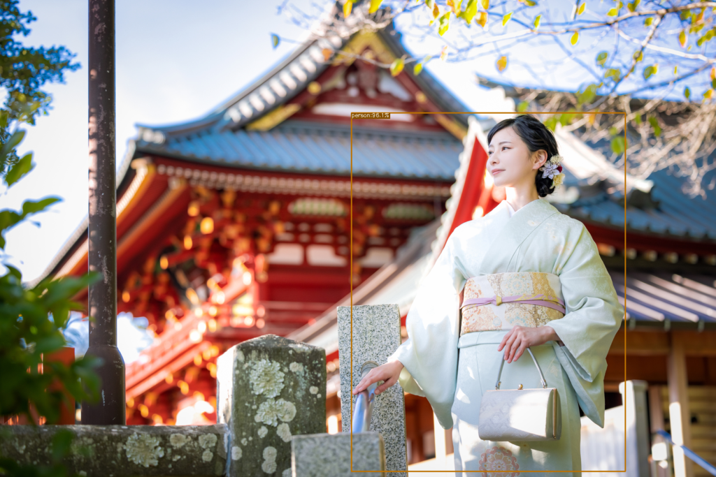
この結果に対して出力結果を表示します。
result = []
[result.extend((final_cls_inds[x],COCO_CLASSES[int(final_cls_inds[x])],final_scores[x],final_boxes[x][0],final_boxes[x][1],final_boxes[x][2],final_boxes[x][3]) for x in range(len(final_scores)))]
df = pd.DataFrame(result, columns = ['class-id','class','score','x-min','y-min','x-max','y-max'])
df| class-id | class | score | x-min | y-min | x-max | y-max |
| 0 | person | 0.961273 | 785.071533 | 252.485382 | 1397.25415 | 1054.818604 |
座標を出力することができました。
この座標を活用して後処理を実装していきます。
Opencvによるモザイク処理
モザイク処理はOpencvにより行うことができます。
画像を一旦縮小してから拡大して、元のサイズに戻すことでモザイク処理が実現します。
縮小するサイズによってモザイクの粗さを調整することができます。
def mosaic(img, alpha):
    w = img.shape[1]
    h = img.shape[0]
    img = cv2.resize(img, (int(w*alpha), int(h*alpha)))
    img = cv2.resize(img, (w, h), interpolation=cv2.INTER_NEAREST)
    return img
YOLOXによるモザイク処理の自動化
これまで紹介したモザイク処理と物体検出を組み合わせます。
先ほど出力した座標を活用します。
input_shape = (640,640)
origin_img = cv2.imread(image_path)
img, ratio = preprocess(origin_img, input_shape)
session = onnxruntime.InferenceSession(model)
ort_inputs = {session.get_inputs()[0].name: img[None, :, :, :]}
output = session.run(None, ort_inputs)
predictions = demo_postprocess(output[0], input_shape)[0]
boxes = predictions[:, :4]
scores = predictions[:, 4:5] * predictions[:, 5:]
boxes_xyxy = np.ones_like(boxes)
boxes_xyxy[:, 0] = boxes[:, 0] - boxes[:, 2]/2.
boxes_xyxy[:, 1] = boxes[:, 1] - boxes[:, 3]/2.
boxes_xyxy[:, 2] = boxes[:, 0] + boxes[:, 2]/2.
boxes_xyxy[:, 3] = boxes[:, 1] + boxes[:, 3]/2.
boxes_xyxy /= ratio
dets = multiclass_nms(boxes_xyxy, scores, nms_thr=0.45, score_thr=0.5)

mkdir(output_dir)
output_path = os.path.join(output_dir, os.path.basename(image_path))
final_boxes, final_scores, final_cls_inds = dets[:, :4], dets[:, 4], dets[:, 5]

for i in range(len(final_scores)):
  xmin = int(final_boxes[i][0])
  ymin = int(final_boxes[i][1])
  xmax = int(final_boxes[i][2])
  ymax = int(final_boxes[i][3])
  origin_img[ymin:ymax,xmin:xmax] = mosaic(origin_img[ymin:ymax,xmin:xmax],0.1)
  print(xmin,ymin,xmax,ymax,final_cls_inds[i])
最後に先ほど定義した関数を実行します。
origin_img[ymin:ymax,xmin:xmax] = mosaic(origin_img[ymin:ymax,xmin:xmax],0.1)
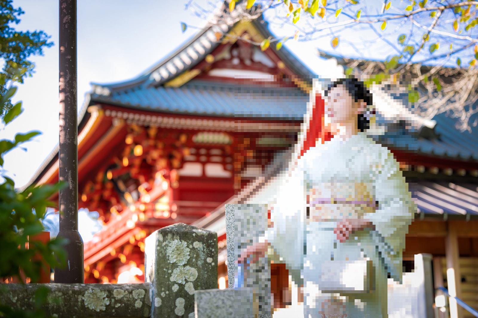
人にモザイク処理を施すことができました。
まとめ
最後までご覧いただきありがとうございました。
今回は、YOLOXの後処理の活用例としてモザイク処理の自動化を実装する方法を紹介しました。
学習済モデルはもちろん、これまで紹介してきた方法で作成したモデルでも使用することが可能です。
YOLOXの活用の幅が広がりそうですね。