このシリーズではE資格対策として、書籍「ゼロから作るDeep Learning」を参考に学習に役立つ情報をまとめています。
<参考書籍>
2層のニューラルネットワーク
はじめに、2層ニューラルネットワークを、一つのクラスとして実装してみます。
class TwoLayerNet:
    def __init__(self, input_size, hidden_size, output_size, weight_init_std=0.01):
        self.params = {}
        self.params['W1'] = weight_init_std * np.random.randn(input_size, hidden_size)
        self.params['b1'] = np.zeros(hidden_size)
        self.params['W2'] = weight_init_std * np.random.randn(hidden_size, output_size)
        self.params['b2'] = np.zeros(output_size)

    def predict(self, x):
        W1, W2 = self.params['W1'], self.params['W2']
        b1, b2 = self.params['b1'], self.params['b2']

        a1 = np.dot(x, W1) + b1
        z1 = sigmoid(a1)
        a2 = np.dot(z1, W2) + b2
        y = softmax(a2)

        return y

    def loss(self, x, t):
        y = self.predict(x)
        return cross_entropy_error(y, t)

    def accuracy(self, x, t):
        y = self.predict(x)
        y = np.argmax(y, axis=1)
        t = np.argmax(t, axis=1)

        accuracy = np.sum(y == t) / float(x.shape[0])
        return accuracy

    def numerical_gradient(self, x, t):
        loss_W = lambda W: self.loss(x, t)

        grads = {}
        grads['W1'] = numerical_gradient(loss_W, self.params['W1'])
        grads['b1'] = numerical_gradient(loss_W, self.params['b1'])
        grads['W2'] = numerical_gradient(loss_W, self.params['W2'])
        grads['b2'] = numerical_gradient(loss_W, self.params['b2'])

        return grads

    def gradient(self, x, t):
        W1, W2 = self.params['W1'], self.params['W2']
        b1, b2 = self.params['b1'], self.params['b2']
        grads = {}

        batch_num = x.shape[0]

        a1 = np.dot(x, W1) + b1
        z1 = sigmoid(a1)
        a2 = np.dot(z1, W2) + b2
        y = softmax(a2)

        dy = (y - t) / batch_num
        grads['W2'] = np.dot(z1.T, dy)
        grads['b2'] = np.sum(dy, axis=0)

        dz1 = np.dot(dy, W2.T)
        da1 = sigmoid_grad(a1) * dz1
        grads['W1'] = np.dot(x.T, da1)
        grads['b1'] = np.sum(da1, axis=0)

return grads2層のニューラルネットワークを実装するためのTwoLayerNetクラスを定義しています。__init__メソッドでは、入力層、隠れ層、出力層のサイズを引数として受け取り、重みとバイアスの初期値を設定します。重みは、標準偏差weight_init_stdのガウス分布によって初期化され、バイアスはゼロで初期化されます。
predictメソッドでは、与えられた入力データxに対するネットワークの出力を計算します。まず、入力層と隠れ層の間のアフィン変換を行い、その結果をシグモイド関数で活性化します。次に、隠れ層と出力層の間でアフィン変換を行い、その結果をソフトマックス関数で活性化して出力を得ます。
lossメソッドでは、入力データxと正解ラベルtを引数に取り、クロスエントロピー誤差を計算して損失を求めます。
accuracyメソッドでは、入力データxと正解ラベルtを用いて、ネットワークの分類精度を計算します。
numerical_gradientメソッドでは、数値微分によって損失関数の勾配を計算します。勾配は、重みとバイアスに対して損失がどの程度変化するかを示す量です。gradientメソッドでは、誤差逆伝播法を用いて効率的に勾配を計算します。この勾配は、ネットワークのパラメータを更新する際に使用されます。
ミニバッチ学習の実装
TwoLayerNetを対象にMNISTデータを使って学習します。
import numpy as np
from keras.datasets import mnist
import matplotlib.pyplot as plt

def identity_function(x):
    return x

def step_function(x):
    return np.array(x > 0, dtype=np.int)

def sigmoid(x):
    return 1 / (1 + np.exp(-x))

def sigmoid_grad(x):
    return (1.0 - sigmoid(x)) * sigmoid(x)

def relu(x):
    return np.maximum(0, x)

def relu_grad(x):
    grad = np.zeros_like(x)
    grad[x >= 0] = 1
    return grad

def softmax(x):
    x = x - np.max(x, axis=-1, keepdims=True)
    return np.exp(x) / np.sum(np.exp(x), axis=-1, keepdims=True)

def sum_squared_error(y, t):
    return 0.5 * np.sum((y - t) ** 2)

def cross_entropy_error(y, t):
    if y.ndim == 1:
        t = t.reshape(1, t.size)
        y = y.reshape(1, y.size)

    if t.size == y.size:
        t = t.argmax(axis=1)

    batch_size = y.shape[0]
    return -np.sum(np.log(y[np.arange(batch_size), t] + 1e-7)) / batch_size

def softmax_loss(X, t):
    y = softmax(X)
    return cross_entropy_error(y, t)

def _numerical_gradient_1d(f, x):
    h = 1e-4
    grad = np.zeros_like(x)

    for idx in range(x.size):
        tmp_val = x[idx]
        x[idx] = float(tmp_val) + h
        fxh1 = f(x)

        x[idx] = tmp_val - h
        fxh2 = f(x)
        grad[idx] = (fxh1 - fxh2) / (2 * h)
        x[idx] = tmp_val

    return grad


def numerical_gradient_2d(f, X):
    if X.ndim == 1:
        return _numerical_gradient_1d(f, X)
    else:
        grad = np.zeros_like(X)

        for idx, x in enumerate(X):
            grad[idx] = _numerical_gradient_1d(f, x)

        return grad

def numerical_gradient(f, x):
    h = 1e-4
    grad = np.zeros_like(x)

    it = np.nditer(x, flags=['multi_index'], op_flags=['readwrite'])
    while not it.finished:
        idx = it.multi_index
        tmp_val = x[idx]
        x[idx] = tmp_val + h
        fxh1 = f(x)

        x[idx] = tmp_val - h
        fxh2 = f(x)
        grad[idx] = (fxh1 - fxh2) / (2 * h)

        x[idx] = tmp_val
        it.iternext()

    return grad

class TwoLayerNet:
    def __init__(self, input_size, hidden_size, output_size, weight_init_std=0.01):
        self.params = {}
        self.params['W1'] = weight_init_std * np.random.randn(input_size, hidden_size)
        self.params['b1'] = np.zeros(hidden_size)
        self.params['W2'] = weight_init_std * np.random.randn(hidden_size, output_size)
        self.params['b2'] = np.zeros(output_size)

    def predict(self, x):
        W1, W2 = self.params['W1'], self.params['W2']
        b1, b2 = self.params['b1'], self.params['b2']

        a1 = np.dot(x, W1) + b1
        z1 = sigmoid(a1)
        a2 = np.dot(z1, W2) + b2
        y = softmax(a2)

        return y

    def loss(self, x, t):
        y = self.predict(x)
        return cross_entropy_error(y, t)

    def accuracy(self, x, t):
        y = self.predict(x)
        y = np.argmax(y, axis=1)
        t = np.argmax(t, axis=1)

        accuracy = np.sum(y == t) / float(x.shape[0])
        return accuracy

    def numerical_gradient(self, x, t):
        loss_W = lambda W: self.loss(x, t)

        grads = {}
        grads['W1'] = numerical_gradient(loss_W, self.params['W1'])
        grads['b1'] = numerical_gradient(loss_W, self.params['b1'])
        grads['W2'] = numerical_gradient(loss_W, self.params['W2'])
        grads['b2'] = numerical_gradient(loss_W, self.params['b2'])

        return grads

    def gradient(self, x, t):
        W1, W2 = self.params['W1'], self.params['W2']
        b1, b2 = self.params['b1'], self.params['b2']
        grads = {}

        batch_num = x.shape[0]

        a1 = np.dot(x, W1) + b1
        z1 = sigmoid(a1)
        a2 = np.dot(z1, W2) + b2
        y = softmax(a2)

        dy = (y - t) / batch_num
        grads['W2'] = np.dot(z1.T, dy)
        grads['b2'] = np.sum(dy, axis=0)

        dz1 = np.dot(dy, W2.T)
        da1 = sigmoid_grad(a1) * dz1
        grads['W1'] = np.dot(x.T, da1)
        grads['b1'] = np.sum(da1, axis=0)

        return grads

(x_train, t_train), (x_test, t_test) = mnist.load_data()
x_train = x_train.reshape(x_train.shape[0], -1)
x_train = x_train.astype('float32') / 255
x_test = x_test.reshape(x_test.shape[0], -1)
x_test = x_test.astype('float32') / 255

t_train = np.eye(10)[t_train]
t_test = np.eye(10)[t_test]

network = TwoLayerNet(input_size=784, hidden_size=50, output_size=10)

iters_num = 10000
train_size = x_train.shape[0]
batch_size = 100
learning_rate = 0.1

train_loss_list = []
train_acc_list = []
test_acc_list = []

iter_per_epoch = max(train_size / batch_size, 1)

for i in range(iters_num):
    batch_mask = np.random.choice(train_size, batch_size)
    x_batch = x_train[batch_mask]
    t_batch = t_train[batch_mask]

    grad = network.gradient(x_batch, t_batch)
    for key in ('W1', 'b1', 'W2', 'b2'):
        network.params[key] -= learning_rate * grad[key]

    loss = network.loss(x_batch, t_batch)
    train_loss_list.append(loss)

    if i % iter_per_epoch == 0:
        train_acc = network.accuracy(x_train, t_train)
        test_acc = network.accuracy(x_test, t_test)
        train_acc_list.append(train_acc)
        test_acc_list.append(test_acc)
        print("train acc, test acc | " + str(train_acc) + ", " + str(test_acc))

import matplotlib.pyplot as plt

# グラフの描画
markers = {'train': 'o', 'test': 's'}
x = np.arange(len(train_acc_list))
plt.plot(x, train_acc_list, label='train acc')
plt.plot(x, test_acc_list, label='test acc', linestyle='--')
plt.xlabel("epochs")
plt.ylabel("accuracy")
plt.ylim(0, 1.0)
plt.legend(loc='lower right')
plt.show()
実行結果:
train acc, test acc | 0.10441666666666667, 0.1028
train acc, test acc | 0.7821833333333333, 0.7884
train acc, test acc | 0.8787833333333334, 0.8819
train acc, test acc | 0.8991833333333333, 0.9024
train acc, test acc | 0.9089666666666667, 0.9123
train acc, test acc | 0.9154833333333333, 0.9178
train acc, test acc | 0.9207666666666666, 0.9215
train acc, test acc | 0.9244, 0.9251
train acc, test acc | 0.92845, 0.928
train acc, test acc | 0.93175, 0.9297
train acc, test acc | 0.9349, 0.9349
train acc, test acc | 0.9375166666666667, 0.9366
train acc, test acc | 0.9389833333333333, 0.9386
train acc, test acc | 0.9416166666666667, 0.9411
train acc, test acc | 0.9426833333333333, 0.9412
train acc, test acc | 0.94485, 0.9436
train acc, test acc | 0.9466833333333333, 0.9439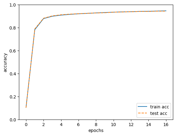
まず、必要なライブラリ(numpy, keras, matplotlib)をインポートし、活性化関数や損失関数を定義しています。具体的には、恒等関数、ステップ関数、シグモイド関数、ReLU関数、ソフトマックス関数、二乗和誤差、交差エントロピー誤差、および勾配計算関数が定義されています。
次に、2層ニューラルネットワークのクラスTwoLayerNetを定義し、その中で重みの初期化、予測、損失計算、精度計算、勾配計算を行うメソッドが実装されています。その後、MNISTデータセットをロードし、学習用データとテスト用データに分割しています。データは、各画像を784次元のベクトルに変換し、正規化してから使用しています。
ニューラルネットワークのインスタンスを作成し、学習を開始します。学習は10000回のイテレーションを行い、各イテレーションでランダムに選択されたミニバッチを用いて勾配降下法によってパラメータを更新しています。各エポックの終わりに、学習データとテストデータの精度を計算し、結果をリストに保存しています。最後に、matplotlibを使用して学習データとテストデータの精度をグラフに描画して表示しています。
ミニバッチ学習
このコードでは、ミニバッチ学習を用いてニューラルネットワークの学習を行っています。
ミニバッチ学習とは、訓練データからランダムに一部のデータ(ミニバッチ)を選び出し、そのミニバッチを用いて勾配降下法によってパラメータを更新する手法です。この方法は、全データを使ったバッチ学習に比べて計算コストが低く、またオンライン学習(1つのデータごとにパラメータを更新する手法)に比べて収束性能が良いとされています。
このコードにおけるミニバッチ学習の実装は、以下の部分になります。
- イテレーション数(10000回)を設定しています。
- 各イテレーションで、訓練データからランダムに選択されたミニバッチ(サイズ100)を取得しています。
- そのミニバッチを用いて、ニューラルネットワークの勾配を計算し、パラメータを更新しています。
エポック
エポックとは、学習において訓練データ全体を1回すべて使い切ることを指します。つまり、1エポックが終わると、訓練データ全体が1回学習に使用されたことになります。エポック数を増やすことで、学習がより進み、モデルの性能が向上することが期待されますが、過学習のリスクも高まります。
このコードにおけるエポックの実装は、以下の部分になります。
- 訓練データサイズとミニバッチサイズから1エポックあたりのイテレーション数(
iter_per_epoch)を計算しています。 - イテレーションごとに、現在のイテレーションがエポックの境界(
i % iter_per_epoch == 0)であるかどうかを判定しています。 - エポックの境界である場合、学習データとテストデータの精度を計算し、結果をリストに保存しています。
エポックを用いることで、定期的にモデルの性能を把握し、適切な学習回数を決定することができます。また、過学習の兆候を検出するためにも役立ちます。
まとめ
最後までご覧いただきありがとうございました。